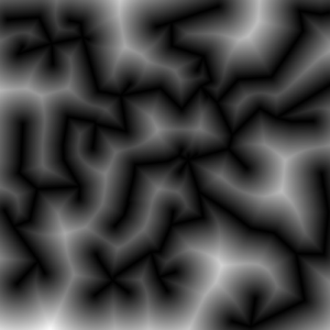
First of all: what is the gain of using distance fields for terrain generation? A distance field is the image of a distance function where black is very close to some object and white is far away. The results differ for different shaped objects as points or lines.
Well, using a 2D distance field as a 2D height map will create mountains or bubbles or cells depending on the objects' shape and the distance function to the objects. Everything in this post is using the euclidean distance  .
.
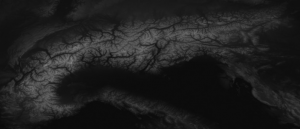
As I had seen a picture like the one on the right side first I had thought "It looks like a mountain".
The second thing I observed was that minimal spanning trees (MST) of point sets where all points are connected to each other looks very much like a maintain ridge chain.
The nice thing you can see on the right picture is that the distance field is "height" where much space is available. So there are height and small mountains mixed and the result is a nice base shape for a terrain.
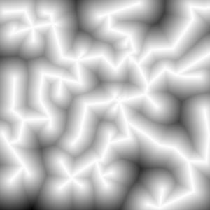
One problem of using a distance function is that outside (not on the image) the distance will increase further and further. So the mountains do end in a plane but in a limited high plateau around the MST region. This leads to the idea of using the inverse:  .
.
An advantage of the inverse function is that our initial points are now the highest points = summits. On the other hand the whole MST has the same height! All ridges and summits are on the same level now. Before all valleys had a height of 0 which was less visible.
Consider the nice property that the points are the summits. It is now very intuitive to give each point an individual height and somehow change the distance function.
All test to change the distance function itself produced artifacts. It will always make problems because the result is a global property which may depend on all vertices and edges of the MST graph.
To solve that issue I took a global interpolation scheme to compute the local height and multiplied the results with the pure distance field which works great!
Computation of the distance field
There are lots of papers related to this issue. Assuming point objects everywere and make a straight forward convolution of a  map would take
  time. There are better ways to do that with a point map, but I thought about using the graph itself. Then the computation takes
  where
where  is the number of edges in the MST which I assumed to be relatively small. It is not possible to go beyond
  because we have to write each pixel at least once. For an implementation example of a point-line distance function see my collection of functions (TODO).
To compute the parametrised height I used a weighted mean:

where
 is a radial basis function. The farther the point is away the less it contributes to the current height. I found the Gaussian RBF and the Inverse Quadric RBF to be useful.
|
1 2 3 4 5 6 7 8 9 10 11 12 13 14 15 16 |
// Use a global interpolation to generate a height for a certain point static float computeHeight(const OrE::ADT::Mesh* mst, float x, float y) { // Calculate a weighted sum of all heights where the weight is the radial basis function. auto it = mst->GetNodeIterator(); float height = 0; float weightSum = 0; while( ++it ) { const Vec3& vPos = ((PNode*)&it)->GetPos(); //float distance = 1.0f/(1.0f + 2.0f*(sqr(vPos.y-y) + sqr(vPos.x-x))); // Inverse quadric RBF float distance = exp(-0.0006f*(sqr(vPos.y-y) + sqr(vPos.x-x))); // Gaussian height += distance * vPos.z; weightSum += distance; } return height / weightSum; } |


