Author Archives: Johannes

(Hex-Grid) Dungeon Generation II: Population

The first post of this series (Hex-Grid Dungeon Generation I) showed two approaches how to generate a connected cave system on a hex-grid. In this post I will discuss an algorithm for spawning things (enemies, chests, ...). The same algorithm can be applied multiple times for different kinds of entities, or in each spawn event random choices can be made.

First, I want to introduce some criteria which I required for the algorithm:

  1. Poisson-disc: Spawned entities should not cluster randomly. This gives more control over the difficulty of the dungeon. Lets say minClearanceRadius  is the distance in which we have no other entities.
  2. Space: each entity should be surrounded by enough free (ground) tiles. This allows to place specific entities like the boss in larger areas. Let spaceRadius  be the radius in which we count the free tiles and minSpace  the number of those tiles which should be free.
  3. Minimum number: make sure there are at least forceNum  entities.

Poisson-disc Sampling (1.)

Poisson-disc sampling produces points that are tightly-packed, but no closer to each other than a specified minimum distance. -- Jason Davis [Dav]

There are numerous scientific works on the problem of Poisson-disc sampling in many dimensions [Bri07] or on triangulated meshes [CJWRW09], [Yuk15] just to name a few. However, the problem gets much simpler in our case. We have a discretized map and each tile is either part of the output set or not. A simple algorithm is

Here, validTiles.getRandom()  is very easy to implement, if our set is a Hash-Set. Then, we can simply take the first element returned by some iterator. The foreach loop is pseudo-code to a high degree. It even has some degree of freedom by defining the distance. One choice would be to iterate over the neighborhood like described on [Pat13]. Another is to use geodesic distances, i.e. all tiles whose shortest path to the newPosition  is smaller or equal the minClearanceRadius .

I implemented the second distance variant: Taking only tiles which are reachable in  minClearanceRadius+1 steps, allows close but non-connected caverns to be independent of each other. E.g. if we have multiple parallel corridors they do not influence each other. Using Dijkstra's Algorithm we can even use a custom cost function to achieve this ranged based iteration.

Space condition (1. + 2.)

To add the second condition to the algorithm we need to modify the initialization only. Instead of taking all tiles we can only add those with enough free ground tiles around them to fill validTiles .

If you want to implement a relative threshold dependent on the radius, here are the formulas for the number of tiles in a radius of r  for different types of grids:

  • Hex-Grid:
  • Quad-Grid with 8 neighborhood:
  • Quad-Grid with 4 neighborhood:

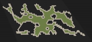
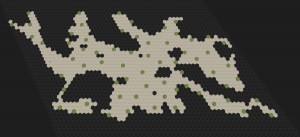
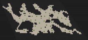
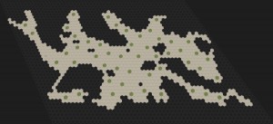
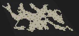
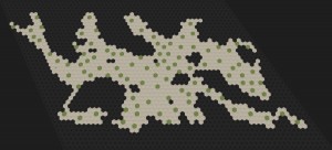
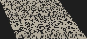
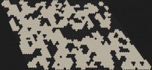
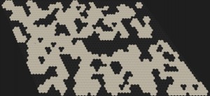
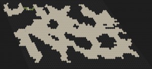
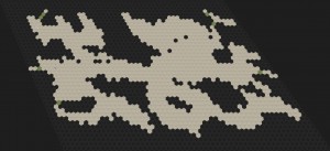
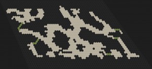
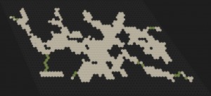
Lets have a look at some results: The images show: all tiles which fulfill the space condition, a sampling with (1.) but not (2.) and two variants fulfilling both properties. The number of generated entities depends on the random picking from the valid set. There can be regions which are sparsely populated because two relative distant entities block the entire area. Other algorithms solve this by placing new elements on the wave front of a breadth-first search.

space_r1

Tiles with full space in range 1

poisson_66entities

No (2.) - 66 entities

poisson_42entities

(1.) + (2.) - 42 entities

poisson_50entities

(1.) + (2.) - 50 entities

Soft Constraints (1. + 2. + 3.)

While the above algorithm meets requirements 1. and 2. easily it can happen that there is none or to few tiles which fulfill both properties. In some crucial cases (e.g. the boss) this may lead to invalid dungeons at all - just because there was one space to few.

Solving all three problems together is much more difficult. I decided to add a priority queue to get the best remaining tile according to a cost for violations of 1. and 2. The final cost function I came up with is
.
The terms are divided by the maximum values to be in the same range, so the add balances between the two.

The real problem is now to maintain this cost function and the queue. Whenever we spawn an entity we want to recompute the cost for all tiles in range. To do so we need to find the elements. There are two possibilities: iterate over the entire queue, update and then call heapify, or somehow access the specific elements. The final choice should depend on whatever is smaller (number of elements in queue or neighborhood). To find the elements fast I have implemented a combined HashSet-PriorityQueue which can be found in my github repository. The idea is that whenever one of the two data structures moves an element it tells the other one. Both keep the indices into the adjoint data structure, but only one contains the real elements. In my case the heap consists of indices in the hash set only (so restoring heap property is cheap). The hash set is quite usual and contains a heap index besides the data.

Another branch of the same repository (map-master) also contains the two populate  algorithms described in this post. The results of the final algorithm are shown in the next two images:

Priority based sampling: 75 entities forced

Priority based sampling: 75 entities forced

aes

Priority based sampling: 100 entities forced

The quality on the right side does not look optimal, but there are twice as much elements as without the forcing! While there is room for improvements (e.g. using diffusion) I think the algorithm is good enough (and easy controllable) to produce enemies and loot in dungeons.

[Pat13] Amit Patel, http://www.redblobgames.com/grids/hexagons/, 2013
[Dav] Davies Jason, https://www.jasondavies.com/poisson-disc/
[Bri07] Robert Bridson, Fast Poisson Disk Sampling in Arbitrary Dimensions, 2007
[CJWRW09] D. Cline, S. Jeschke, K. White, A. Razdan and P. Wonka, Dart Throwing on Surfaces, 2009
[Yuk15] Cem Yuksel, Sample Elimination for Generating Poisson Disk Sample Sets, 2015

Hex-Grid Dungeon Generation I

This is the first new post for a series of dungeon generator experiences. As you might expect I have a new game project (since February this year) which is based on a hex-gird. The game mechanic will be something between Hack-n-Slay and Pokémon, but more to that on a dedicated project page later.

First, there is an extremely valuable source for many algorithms appearing on a hex grid: http://www.redblobgames.com/grids/hexagons/ [1]. This side is one of the best web pages I have seen so far. It has very helpful explanations for all hex-grid problems and shows interactive examples for each of them. Moreover, if you change an option in one example, all others adapt to this same option. If you don't understand a detail in this post related to the hex-grid, just have a look on the mentioned side.

Generating Caves on Hex-Grids (Cellular Automaton)

There are many types of dungeons and generators, especially on quad-grids. You can have special maze generators, room based dungeons and caves. This post shows how to generate caves on the hex-grid.

Cellular automata seem to be the most common approach for generating caves. One source I found inspirational is this article [2]. However, I was not able to find sources on good hex-grid cave generator rules quickly, so I started experimenting and here are my results.

The basic idea is to start with a random initialization (floor/wall) and apply some iterations of a cellular automaton. This automaton will check the neighborhood of a cell and decide which type the cell gets in the next turn, based on the number of certain elements in the vicinity. Let being the count of Floor (or Wall) tiles around a cell within a range of 1 excluding the tile itself. This count can be a number in . Then, the following rules produced good cave maps:

One important thing is when and how the new type is set. Usually, an automaton would change all states at once, after the types of all cells are determined. Directly changing the cell type will also change the neighborhood of the next cell, which can lead to a fast collapse into a single type only. Luckily the above rule handles direct changes very well. So, yes I am changing types immediately...

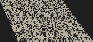
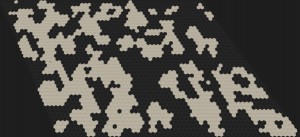
Here are two examples with different initialization conditions (60% and 65%), using the same seed. Each row shows the initialization and two iterations.

cave_init60 cave_60_it1 cave_60_it2
cave_init65 cave_65_it1 cave_65_it2

The base shape is determined by the simple fact that I loop over my memory in a rectangle fashion during initialization. It could easily be changed, but I see no need for it. Using the 65% initialization I did not see any caves with large disconnected components on several seeds. If a dungeon is too small it can thus be regenerated with a high success probability. However, even through there are only a few small disconnected components we want to remove them before proceeding with populating the dungeon. It would be a disaster if the boss is in another component and the only way out of a dungeon is killing that boss... Extracting a single component is simply by using a flood-fill.

To make sure we know a good start point, we can modify the initialization. For example, I set all seven tiles around position (0,0) to floor. This gives an area of high floor density which will lead to even more floor tiles in the automaton iteration. It is more likely that the region grows than that it shrinks.

Fractal Noise as Generator

While the above rule is relatively stable, there are no real options to tweak the scale, ... Instead of trying to resample the map as done by [2] to get larger caves I switched to another idea: Generating a fractal noise (Value Noise or Perlin Noise) and using a threshold to determine occupied tiles. Assuming the fractal noise is in [0,1] a threshold of 0.5 should give roughly 50% occupancy. There are several degrees of freedom:

  • The threshold: steers how much of the map is occupied (sparsity)
  • The number of octaves: large scale vs. small scale structures
  • The turbulence function (adding octaves, multiplying, ridged (abs), ...): different shapes

As noise function I used a Perlin Noise with ridged turbulence function. Unfortunately, any noise results in very straight boundaries at the edge of the generation area. Therefore, I gradually increase the threshold to the outer boundary (quadratic over radius of 10 tiles) up to 1.

Of course, there is now guarantee for connected components, but this is the same as for the cellular automaton. I decided to fix this problem with a general approach described in the next section. But, first here some examples of the generator output.  The images have increasing threshold levels which reduces the number of non-empty tiles and increases the chance for non-connected components. The green connections are created by the algorithm below.

cave_perlin_1 cave_perlin_4 cave_perlin_6 cave_perlin_7

Reconnecting Components

Rather than recreating dungeons until they have the right size by accident it is better to somehow increase connectivity. Starting with some known (e.g. (0,0) start position) or a random floor tile one can mark all connected tiles with a flood fill. Then, another unmarked tile can be searched and connected with a randomized work between the start region and the obviously disconnected region. I use an A* way search where empty tiles have a random high cost in [5,20] (fixed for the time of search) and floor tiles have a low constant cost [0.01]. This leads to a non-straight connection between probably close points of the two sets. After connecting the two regions the new part can be marked the same way as the start region (it now belongs to it). When using a simple scan-line as search, all disconnected components will be connected finally.

[1] http://www.redblobgames.com/grids/hexagons/
[2] http://www.roguebasin.com/index.php?title=Cellular_Automata_Method_for_Generating_Random_Cave-Like_Levels

Numerical Recipes for Rendering

Until recently, I usually ignored floating point arithmetic errors in my applications. In graphics you are naturally interested in speed and what does it matter if an object is translated wrongly a thousands part of a pixel? On the other hand: how hard can it be to test if a point lies within a sphere? As formula this is very straight forward: len(center-point) <= radius. Unfortunately this operation involves a sum of squares and the rounding errors indeed lead to wrong classifications. I don't even know how to test if a point is inside a sphere correct without unlimited precision math.

This is a post about different tricks and algorithms to avoid numerical issues. Especially in ray casting and intersection methods I got some artifacts in the past. Many of them occurred to me while writing my math and intersection library Epsilon.

Most of the knowledge here is drawn from the article "What Every Computer Scientist Should Know About Floating-Point Arithmetic" [Go91] and some other articles. I will not go as deep as the linked articles. Instead I will collect what are the most useful algorithms and show some examples when it makes sense to use them. Also, I won't go into details of why there is a numerical issue - for that I recommend to read [Go91].
In the graphs below I computed the relative error of the respective expressions. This is calculated as the result minus the true result divided by the true result, i.e. abs((x-ref)/ref). Thereby, the true result is computed using the most correct expression in double precision.

Rounding

Rounding is the root of all evil. Floats have the nice property that they always have (more or less) the same relative precision. That means, it doesn't matter if a number is small or huge, as long as it is not too small (underflow) or too large (overflow). Still, the number of digits is limited. Lets assume we have 3 digits precision in decimal system, than adding 100e1 and 1 gives 100e1. So the 1 had no effect at all, since the true result 1001 was rounded to three digits. In most cases the rounding during addition is not fatal, because the error is relatively small (all 3 stored digits are correct). Addition and subtraction may only have an error in the last digit, i.e. they will not be far away from the true result. If rounding to the closer number the error is at most 0.5 ulp (units is the last place).

The point where rounding makes things bad is if errors accumulate. In the worst case catastrophic cancellation can happen, where a subtraction of similar numbers reveals a previous error. An example from [Go91]: Again we have decimal numbers with 3 digits: a=1.22, c=2.28, b=3.34  and want to compute b*b-4*a*c. The exact result is 0.0292. In limited precision it is b*b=11.2 (0.5 ulp), 4*a*c=11.1 (0.5 ulp) and finally 0.1 (70 ulp !).

1-x² and x²-y²

Lets start with the 1_squareXsmallest term.  1-x*x is very useful in trigonometric expressions, since sin^2 + cos^2 = 1. For example: this can be used for the compression of normal vectors in polar coordinates. So, what is the problem of this expression?
It is catastrophic cancellation, because x is squared and then subtracted, which is the most basic example where this kind of error occurs.
It is possible to write the expression using the third binomial formula (1-x)*(1+x), which is more robust. This form has a bigger error in general, but as the graph shows, its error does not increase if both numbers are very similar and is very small otherwise. However, a maximal error of 0.012% in the first form is not that dramatic for most applications.
Note, that the same trick applies to x*x-y*y  which can be reformulated to (x-y)*(x+y)

Quadratic Equation

squarepolyrootsThere are many algorithms which require the roots of a quadratic polynomial, e.g. a ray-sphere intersection. The basic expression we want to solve is ax² + bx + c = 0 for which the known solution is

If the term below the root gets wrong (like in the example above) this is not that bad, because if that happens the result is small compared to b. Now, the problem occurs again if b and the square root are similar and get subtracted. However, this is only the case for one of the two results, because the other one adds the root term. The graph shows that if b is 1000 times larger than a and c the error becomes already larger than 10% (for 32bit floats). For a factor over 6000, rounding toggles between 100% and some smaller error for odd and even numbers.
Again, it is possible to use the third binomial formula and multiply the term with the denominator using the inverted sign [X05]:

Note, that the changed and we get the subtraction for the two results reversed. A stable implementation needs to check which of the two formulas is better for which x and than use one of the two different terms.

ln(1+x) and exp(1+x,n)

log1pFor small |x|, 1+x discards many digits, so both expressions will be inaccurate. The later can be useful in numerical integrations (e.g. simulation of movement), when there is a grow or decrease over time. It can be expressed using the first one: exp(1+x,n) = exp(n*ln(1+x)) which leaves us with the problem of ln(1+x) to be inaccurate. Well, if you look at the graph it is not thaaat important. x must be really close to zero, before something bad happens.

The following code snipped solves this issue. Effectively, the function is multiplied with x/x, where the denominator is replaced by (1+x)-1, which is an estimation of the error made by the summation. [HP82]

You can find a numerical stable log1p method in the math.h (at least in my cpp standard library). Surprisingly, it is slower by a factor of 7 and calls modf, acosf, fdtest and log internally. Seems to be some series expansion inside.

Sum and Variance of Many Numbers

Especially path tracing and other Monte Carlo light transport simulations rely on the law of large numbers. I.e. they converge to the correct result for sufficient many samples. Well, they should, but due to floating point they never will.

First, I experimented with plausible series of 10,000 and 100,000 samples of uniform and exponential distributions. All had shown a systematic underestimation with up to 0.001% error. This is only a problem, if many larger numbers with small variance are added (e.g. for being a uniform sample) which I did not test, because this is not really likely for rendering applications. Still, I will add a few solutions for completeness. See [Wiki1] and [He05] for more alternatives. The first well known solution is the Kahan summation. It tracks the lost digits in a second register to achieve a constant error bound (trivial summation has an error in the number of samples). However, adding doubles naively is already more precise than Kahan summation with two floats, so it makes only sense if we want to have even more precision than double [Wiki1] or cannot use double (e.g. on GPU).

Another option is to recursively compute partial sums. This is quite nice, because computing prefix sums (e.g. for summed area tables) with a parallel algorithm is already more accurate than a linear algorithm.

Beyond the sum of samples we could also be interested in there variance. This time errors can get worse, because if the mean is close to the (with a small variance) we subtract two similar numbers.

Another problem with the naive formulation is, that we need to keep all samples to compute once we know . Both problems are solved by Welford's method explained on [Co08]. I like it, because we don't need to store more than three values which we do anyway (mean, variance and number of samples).

varianceCompared to the often used sum of squares method, which stores x, x*x and n, Welford's algorithm performs much better. In the experiment I used n samples uniformly distributed in [0.5, 1.5] which should be comparable stable (see summation above).
Unfortunately, for more than ~45000 samples the variance in the naive sum of squares method gets negative. Even in the absolute value the error gets larger than 1000% (logarithmic scale!). Besides that catastrophe, all other values have acceptable errors in the 5th to 7th decimal place.

Final Thoughts

I tested a set of recipes for numerical stable computations to see which of them are really necessary in the context of rendering and simulation. Before, I encountered problems in a ray tracing application using ellipsoids leading to geometry misses in my bounding volume hierarchy. So, of course I think using the more stable solution of the quadratic polynomial is a good idea.
Using the third binomial formula is not really necessary, but since it barely changes instruction count/performance it can be used everywhere without thinking.
In the cases of logarithmic functions and summing numbers, errors happen in extremal cases mainly. As long as we do not run into these, which is unlikely in rendering, nothing bad happens with the naive approaches.
However, when using the sums of numbers in some subtraction, as for the computation of variance, I strongly recommend to use a better method. Especially, for unbiased Monte Carlo integration simply adding floats is not enough.

[Co08] Accurately Computing Running Variance, John D. Cook, 2008
http://www.johndcook.com/blog/standard_deviation/
[Co14] Avoiding Overflow, Underflow, and Loss of Precision, John D. Cook, 2014
http://www.codeproject.com/Articles/25294/Avoiding-Overflow-Underflow-and-Loss-of-Precision
[Go91] What Every Computer Scientist Should Know About Floating-Point Arithmetic, David Goldberg, 1991
http://docs.oracle.com/cd/E19957-01/806-3568/ncg_goldberg.html
[HP82] HP-15C Advanced Functions Handbook, Hewlett-Packard Company, 1982
[He05] Binary floating point summation accurate to full precision (Python recipe), Raymond Hettinger, 2005
http://code.activestate.com/recipes/393090/
[Wiki1] https://en.wikipedia.org/wiki/Kahan_summation_algorithm
[X05] 2005, http://people.csail.mit.edu/bkph/articles/Quadratics.pdf