Example Rule: The Redwood Tree

In order to make the core of Voxel Seeds more understandable I would like to explain two generic rules which together create the oak tree.

Each tree is build upon two rules - one for the wood and one for the leaves/needles. Thinking of a real automaton there are much more rules, but considering the form explained in About the automaton behind Voxel Seeds allows branching inside a rule. This is why I refer to generic rules.

As mentioned in the last post about the automaton we added a small memory to each living voxel. The first one was a "Tick" counter. This is some stopwatch when to apply the rule next. Each species has its own intervall length determining the growth speed. Further this counter can be manipulated randomly to break the synchronous growth.

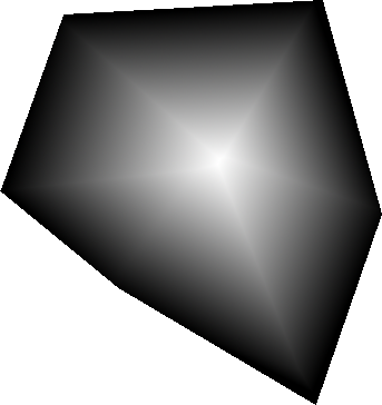
The redwood has the mightiest rule allowing a procedural fractal tree. Lets start with the needles first. The rule is called SphericalLeafRule and is used for oak trees and redwoods. The idea is to seed a center voxel of the needle/leaf type and do a flood-fill of a spherical region. How can the euclidean distance to the center be estimated? This question is answered later for the redwood itself. For needles it is sufficient to use some random manhatten like distance. Therefore the "Generation" memory is used. This is monotonously increasing and the growth stops if the number gets too large. Here is some pseudo code of the rule:

To compute the euclidean distance to some center voxel a little bit more work has to be done. It is possible to store a relative position into a single 32 bit integer value. So one of the two memories could be used to store the center's position relative to the current voxel. If a new voxel is created in the neighbourhood it is easy to add or subtract one from the position to compute the new relative position. With this information each voxel can compute its euclidean distance to some source or destination point.

Now we have the ingredents for a  
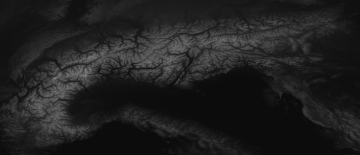
RedWoodRule . First of all the "Generation" can be used to distinguish voxels of the same type but with a different growth behavior. The first important type is the kernel voxel c. The trunk and each branch consists of one line of these. When spawning a new kernel voxel it gets an encoded target in the "Resource" memory. Afterward these voxels try to reproduce into target direction. This is done randomly where the most probable chosen direction is that where the difference to the target is largest. During that growth new kernel voxels are created tangential to the chosen direction to build branches. If the growth reaches the target it creates a center voxel for the needles.
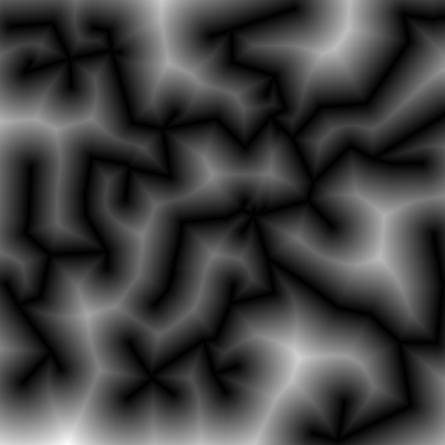
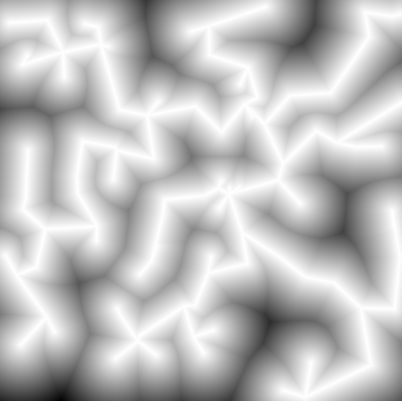
The second type is the raw wood r. These have a "Generation" counter larger than 1000 where the difference to 1000 describes the target width of the trunk/branch. For each kernel voxel the width is determined by the distance to its target. If this width is at least one r voxels are spawned in the neighbourhood. These remember there spawner position in the "Resource" field and growth further if they are not too far away. I.e. if the stored width from the "Generation" counter is larger than there actual euclidean distance. In general this creates a sphere for a single kernel voxel filled with wood. The sum of many such neighboured spheres creates a cylinder. The advantage in contrast to a real cylinder is that twists in the kernel line do not cause holes in the surrounding.

Collision Detection Basics

The basis for all collision detections is analytical geometry. Math can answer the question where two primitives intersect or give the distance between two objects. This post will only cover such basic functions. So it is a collection of primitive - primitive relation functions. There are two functions given. The first only returns collision or not. The second variant returns a resolvement vector. This is a translation vector which have to be applied to object 1 to move the two objects out of each other.

3D

Object Properties
Sphere center , radius
Line start and end , implicit direction
Triangle The 3 vertices in counter clock wise order , implicit normal

Sphere - Sphere

For a detection the distance has to be less or equal to the sum of the radi.

For resolvement just take the connection between the midpoints and the intersection length.

Sphere - Line

First the nearest point on a straight must be computed. If this point does not lie between the start and the end point choose the start or end point respectively.


The resolvement vector is the connection between sphere center and the nearest point on the line.

Sphere - Triangle

The usual way to do this is to project the sphere center to the triangle's plane. Afterwards the barycentric coordinates of the point would be calculated to test if it is inside. If not we still have to test whether the circle from the plane-sphere cut intersects with a triangle or not. Therefore it is sufficient to test the 3 line-sphere cuts because the center is definitely outside. I changed the middle part to hopefully increase the speed. Instead of calculating the barycentric coordinates I compute the closest points on all three sides which I would need in the last step non the less. Then the following condition must be true if the point is inside: the opposite vertex to a side (and therefore a point on that side) must lie on two different "sides" of the projected center. So the dot product of the vectors from the center to a closest point on a triangle-side and to the related triangle-vertex has to be at least 0.

There was one problem when using a full triangle collision in the game Pathfinder. Imagine a box made of triangles. Then the sphere is placed on top near to an edge. The simulation will first push the sphere down. Afterwards the collision detection would report two triangles. The one on the top and one of a side where the sphere collides with a back face. This has the effect that the sphere is pushed away from the edge to the box center on the upper side. To avoid that I use the condition if( fDist < 0.0f || fDist > _S.fRadius ) in lines 10 and 46 instead of if( abs(fDist) > _S.fRadius ) .

The MST Distance Field

Distance field of a convex polygon

Distance field of a convex polygon

First of all: what is the gain of using distance fields for terrain generation? A distance field is the image of a distance function where black is very close to some object and white is far away. The results differ for different shaped objects as points or lines.
Well, using a 2D distance field as a 2D height map will create mountains or bubbles or cells depending on the objects' shape and the distance function to the objects. Everything in this post is using the euclidean distance .
As I had seen a picture like the one on the right side first I had thought "It looks like a mountain".

The second thing I observed was that minimal spanning trees (MST) of point sets where all points are connected to each other looks very much like a maintain ridge chain.

Alps height map (reality)

Alps height map (reality)

Distance to MST of 100 uniform distributed points

Distance to MST of 100 uniform distributed points

The nice thing you can see on the right picture is that the distance field is "height" where much space is available. So there are height and small mountains mixed and the result is a nice base shape for a terrain.

One problem of using a distance function is that outside (not on the image) the distance will increase further and further. So the mountains do end in a plane but in a limited high plateau around the MST region. This leads to the idea of using the inverse: .

Inverse distance of the same MST as in the previous picture

Inverse distance of the same MST as in the previous picture

An advantage of the inverse function is that our initial points are now the highest points = summits. On the other hand the whole MST has the same height! All ridges and summits are on the same level now. Before all valleys had a height of 0 which was less visible.

Consider the nice property that the points are the summits. It is now very intuitive to give each point an individual height and somehow change the distance function.

All test to change the distance function itself produced artifacts. It will always make problems because the result is a global property which may depend on all vertices and edges of the MST graph.

To solve that issue I took a global interpolation scheme to compute the local height and multiplied the results with the pure distance field which works great!

Computation of the distance field

There are lots of papers related to this issue. Assuming point objects everywere and make a straight forward convolution of a map would take time. There are better ways to do that with a point map, but I thought about using the graph itself. Then the computation takes where is the number of edges in the MST which I assumed to be relatively small. It is not possible to go beyond because we have to write each pixel at least once. For an implementation example of a point-line distance function see my collection of functions (TODO).

To compute the parametrised height I used a weighted mean:


where is a radial basis function. The farther the point is away the less it contributes to the current height. I found the Gaussian RBF and the Inverse Quadric RBF to be useful.