The first post of this series (Hex-Grid Dungeon Generation I) showed two approaches how to generate a connected cave system on a hex-grid. In this post I will discuss an algorithm for spawning things (enemies, chests, ...). The same algorithm can be applied multiple times for different kinds of entities, or in each spawn event random choices can be made.
First, I want to introduce some criteria which I required for the algorithm:
- Poisson-disc: Spawned entities should not cluster randomly. This gives more control over the difficulty of the dungeon. Lets say minClearanceRadius is the distance in which we have no other entities.
- Space: each entity should be surrounded by enough free (ground) tiles. This allows to place specific entities like the boss in larger areas. Let spaceRadius be the radius in which we count the free tiles and minSpace the number of those tiles which should be free.
- Minimum number: make sure there are at least forceNum entities.
Poisson-disc Sampling (1.)
Poisson-disc sampling produces points that are tightly-packed, but no closer to each other than a specified minimum distance. -- Jason Davis [Dav]
There are numerous scientific works on the problem of Poisson-disc sampling in many dimensions [Bri07] or on triangulated meshes [CJWRW09], [Yuk15] just to name a few. However, the problem gets much simpler in our case. We have a discretized map and each tile is either part of the output set or not. A simple algorithm is
|
1 2 3 4 5 6 7 8 |
Set validTiles = <all tiles> while(!validTiles.empty()) { newPosition = validTiles.getRandom(); output.add(newPosition); foreach(tile : [distance(newPosition, tile) < minClearanceRadius]) validTiles.remove(tile); } |
Here, validTiles.getRandom() is very easy to implement, if our set is a Hash-Set. Then, we can simply take the first element returned by some iterator. The foreach loop is pseudo-code to a high degree. It even has some degree of freedom by defining the distance. One choice would be to iterate over the neighborhood like described on [Pat13]. Another is to use geodesic distances, i.e. all tiles whose shortest path to the newPosition is smaller or equal the minClearanceRadius .
I implemented the second distance variant: Taking only tiles which are reachable in minClearanceRadius+1 steps, allows close but non-connected caverns to be independent of each other. E.g. if we have multiple parallel corridors they do not influence each other. Using Dijkstra's Algorithm we can even use a custom cost function to achieve this ranged based iteration.
Space condition (1. + 2.)
To add the second condition to the algorithm we need to modify the initialization only. Instead of taking all tiles we can only add those with enough free ground tiles around them to fill validTiles .
If you want to implement a relative threshold dependent on the radius, here are the formulas for the number of tiles in a radius of r for different types of grids:
- Hex-Grid:

- Quad-Grid with 8 neighborhood:

- Quad-Grid with 4 neighborhood:

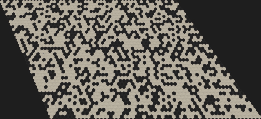
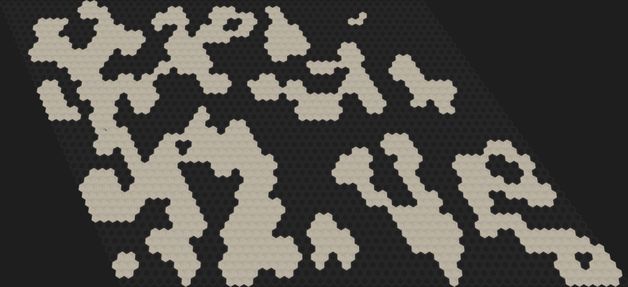
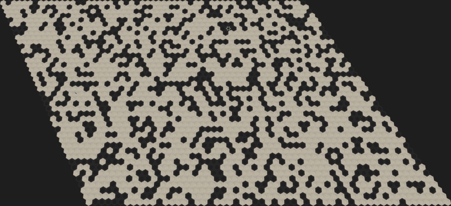
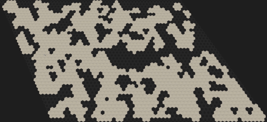
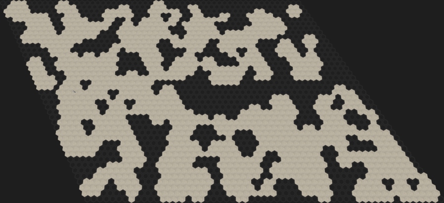
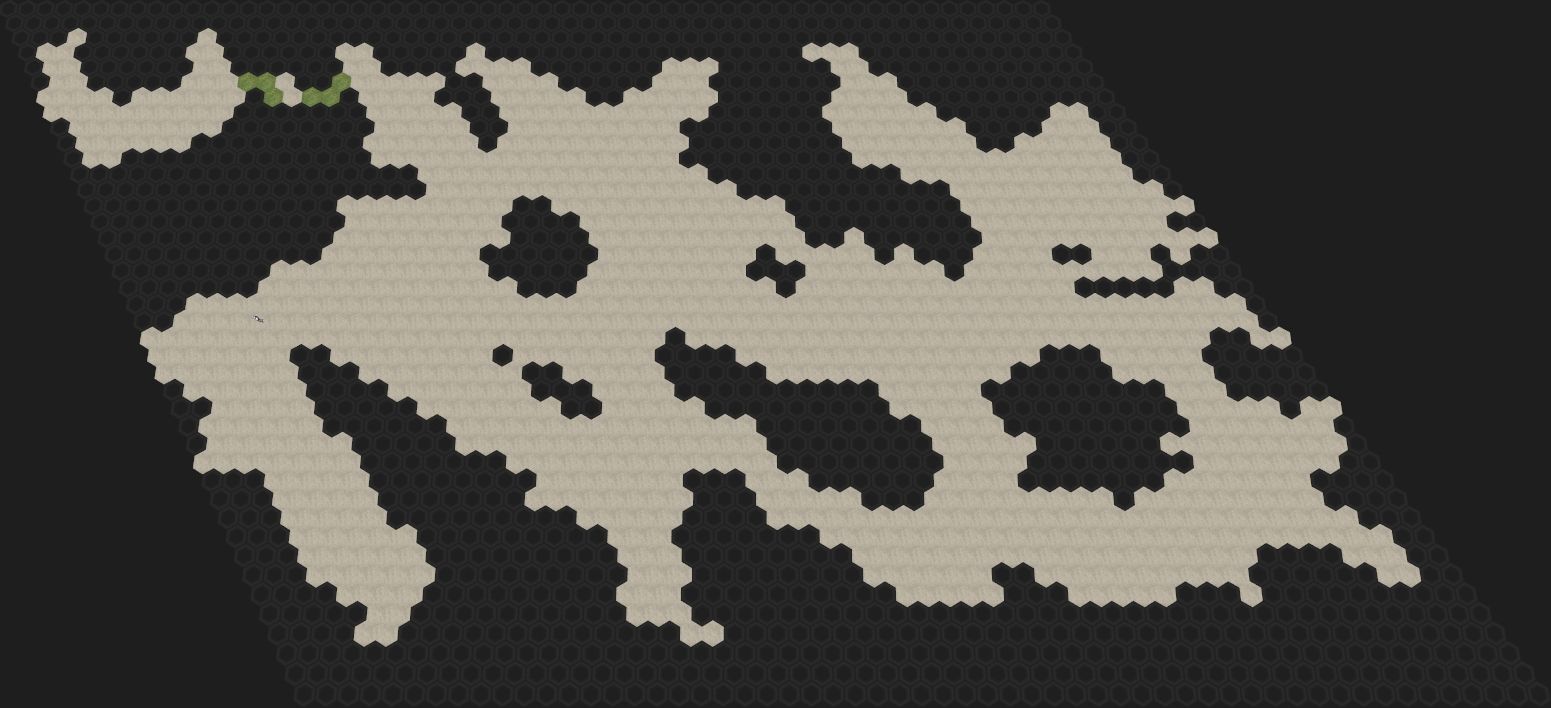
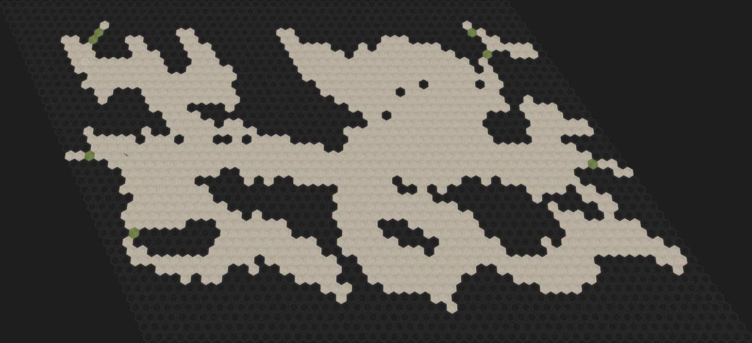
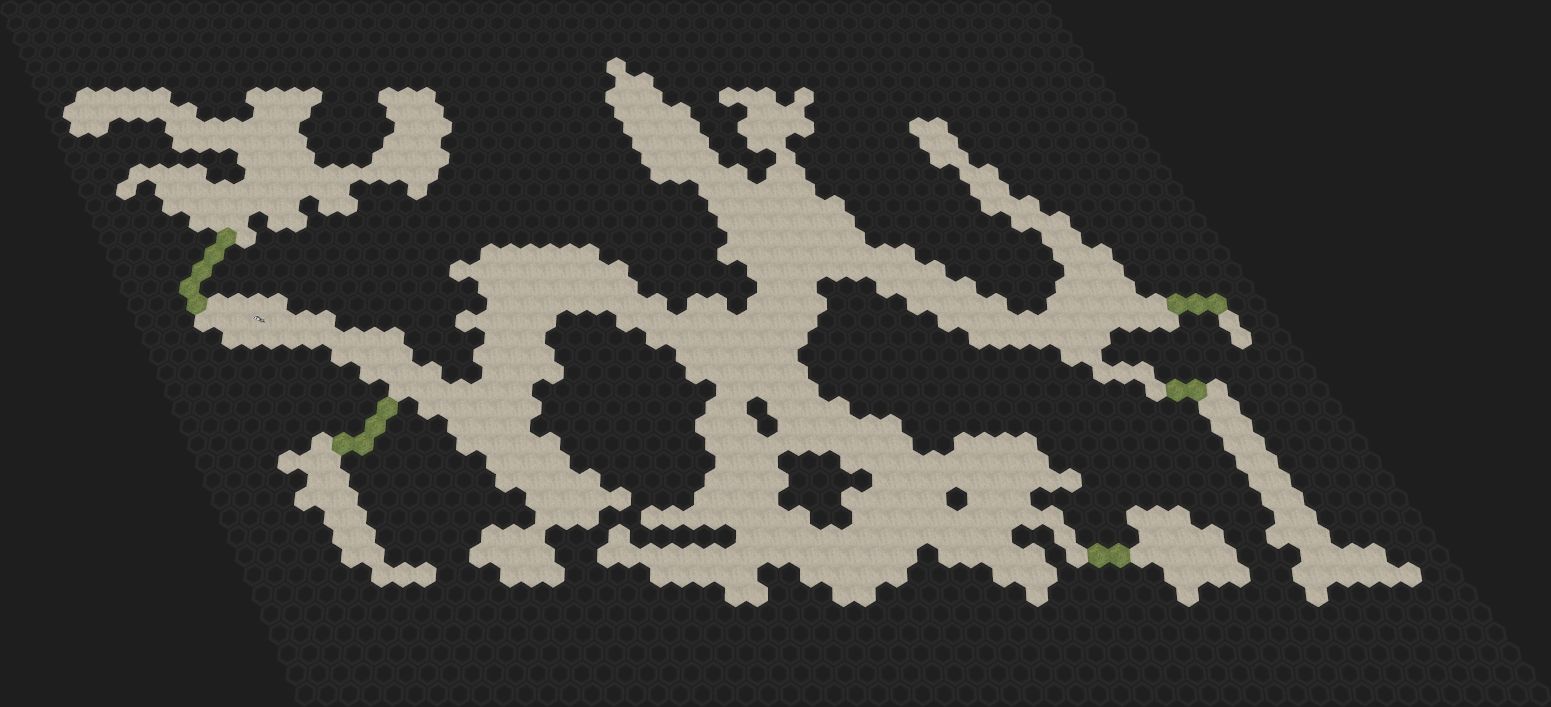
Lets have a look at some results: The images show: all tiles which fulfill the space condition, a sampling with (1.) but not (2.) and two variants fulfilling both properties. The number of generated entities depends on the random picking from the valid set. There can be regions which are sparsely populated because two relative distant entities block the entire area. Other algorithms solve this by placing new elements on the wave front of a breadth-first search.
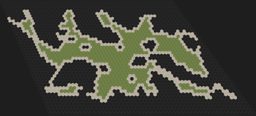 Tiles with full space in range 1 |
 No (2.) - 66 entities |
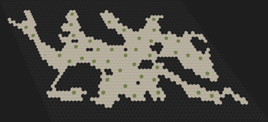 (1.) + (2.) - 42 entities |
 (1.) + (2.) - 50 entities |
Soft Constraints (1. + 2. + 3.)
While the above algorithm meets requirements 1. and 2. easily it can happen that there is none or to few tiles which fulfill both properties. In some crucial cases (e.g. the boss) this may lead to invalid dungeons at all - just because there was one space to few.
Solving all three problems together is much more difficult. I decided to add a priority queue to get the best remaining tile according to a cost for violations of 1. and 2. The final cost function I came up with is
 .
.
The terms are divided by the maximum values to be in the same range, so the add balances between the two.
The real problem is now to maintain this cost function and the queue. Whenever we spawn an entity we want to recompute the cost for all tiles in range. To do so we need to find the elements. There are two possibilities: iterate over the entire queue, update and then call heapify, or somehow access the specific elements. The final choice should depend on whatever is smaller (number of elements in queue or neighborhood). To find the elements fast I have implemented a combined HashSet-PriorityQueue which can be found in my github repository. The idea is that whenever one of the two data structures moves an element it tells the other one. Both keep the indices into the adjoint data structure, but only one contains the real elements. In my case the heap consists of indices in the hash set only (so restoring heap property is cheap). The hash set is quite usual and contains a heap index besides the data.
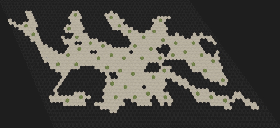
Another branch of the same repository (map-master) also contains the two populate algorithms described in this post. The results of the final algorithm are shown in the next two images:
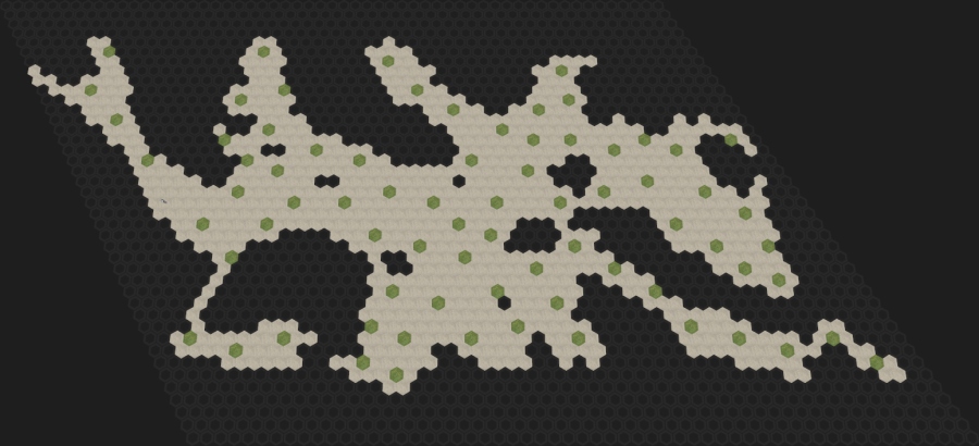 Priority based sampling: 75 entities forced |
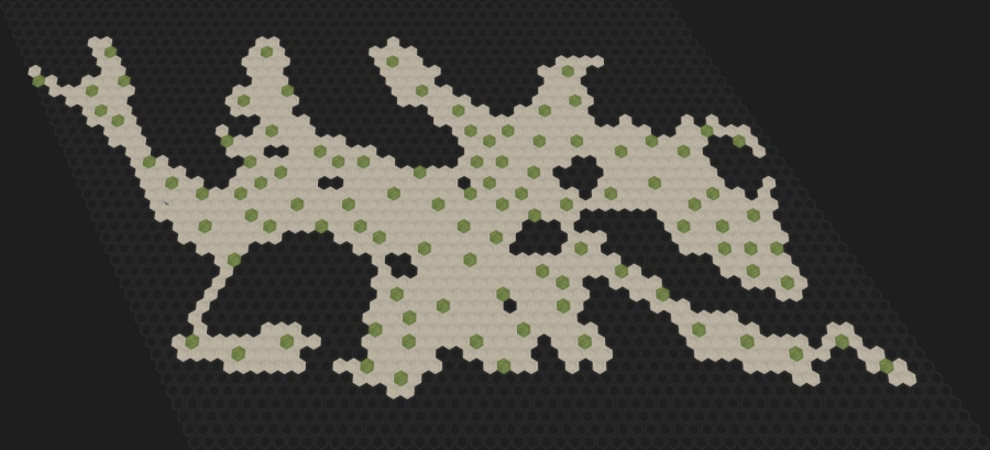 Priority based sampling: 100 entities forced |
The quality on the right side does not look optimal, but there are twice as much elements as without the forcing! While there is room for improvements (e.g. using diffusion) I think the algorithm is good enough (and easy controllable) to produce enemies and loot in dungeons.
[Pat13] Amit Patel, http://www.redblobgames.com/grids/hexagons/, 2013
[Dav] Davies Jason, https://www.jasondavies.com/poisson-disc/
[Bri07] Robert Bridson, Fast Poisson Disk Sampling in Arbitrary Dimensions, 2007
[CJWRW09] D. Cline, S. Jeschke, K. White, A. Razdan and P. Wonka, Dart Throwing on Surfaces, 2009
[Yuk15] Cem Yuksel, Sample Elimination for Generating Poisson Disk Sample Sets, 2015