Here you will find a description of the collision detection for a whole scene in Pathfinder. The post Collision Detection Basics covers the mathematically detection of object - object contacts. The algorithm shown here is designed to be small and efficient at the same time.
An outdoor scene in Pathfinder currently has more than a million polygons. Testing them all for collision would cost far too many operations. So the first thing is to think about a representation of objects for which collision detection can be faster. Easy to see is that the spatial resolution of objects must not as high as there visual representation. A cylinder with 10 edges would not look smooth but behaves well in physics. A closed ten-sided cylinder still consists of 36 triangles. Wouldn't it be better to use an analytic solution for a cylinder? Yes, but it would also make things much more complicated. So I decided to represent everything by spheres and triangles only. Beside the simplification in the polygonal representations one can wrap spheres around everything. Just using a sphere for each object and test against each of this bounding spheres was fast enough that it worked for months. But if you wanna have more than one dynamic object this is not enough.
Common Pruning Approaches
There are different techniques to exclude many objects even without testing against there bounding spheres. Most times a spatial partitioning tree is used. A very famous one is the octree where the space is subdivided into boxes with 8 subboxes each. The objects of the scene are contained in the leaf-boxes which are not further subdivided. Objects which lie in more than one box have to be stored more than once. This causes overhead in the maintainance of the tree which is why I discarded it. For the same reason I did not choose the kd-tree which splits the space along the 3 dimensions recursively.
Another nice approach is the Sweep & Prune technique where all objects are protected to an arbitrary number of axis. Each projection is an interval on one axis which may overlap with the intervals of other objects. Only if the intervals for two objects intersect on all axis they can collide. Due to temporal coherence the change in the projections between two frames is very small and can be computed fast. The drawback is that ray-scene intersections test cannot be improved much with this technique. E.g. a ray with a direction of (1,1,1) (diagonal) would have a maximal projection interval in x-, y- and z-axis direction. From that point of view it would collide with everything. Since ray-scene intersections is something I would like to have I discarded Sweep & Prune too.
My favourite is the hierarchy of bounding volumes. There close objects are grouped and each group has a bounding volume the same way objects already have them. An optimal grouping which creates a balanced binary tree is hard to get, but who says that it must be optimal if it is fast and easy.
The Sphere Tree in Detail
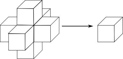
Of course - if I represent everything by triangles and spheres the bounding volumes must be spheres. Other things as boxes could have smaller volumes for the same group but a collision with a sphere is so much faster that ~6 test could be done instead. So lets build a binary tree of spheres.
Construction
One could wait for all objects and build the tree in one big step (offline approach). A good idea would be to search for the two objects where their bounding sphere is the smallest over all pairs. This would create an optimal tree to exclude approximating half of the space in each step in a tree-search. Such an algorithm would take lots of time and only static geometry can be considered at all.
The other way is to insert elements directly to the tree (online approach). Each node of the tree has either two children or is a leaf representing some object. To decide in which branch the new leaf should be inserted test which one would have the smaller bounding volume afterwards. This prefers close and small sub-branches. I will test later if this is a well performing condition (but seems to be good in current benchmarks). A possible alternative would be to use the sphere which growth less.
|
1 2 3 4 5 6 7 8 9 10 11 12 13 14 15 16 17 18 19 20 21 22 23 24 25 26 27 28 29 30 31 |
SphereTreeNode* AddToSphereTree( SphereTreeNode* _pRoot, SphereTreeNode* _pNewLeaf ) { // Is there is nothing the leaf is the tree. if( _pRoot == nullptr ) return _pNewLeaf; // If _pRoot is a leaf create a new intermediate node. if( _pRoot->IsLeaf() ) { ... pNewIntermediate->BoundingSphere = MeldSpheres( _pRoot->BoundingSphere, _pNewLeaf->BoundingSphere ); pNewIntermediate->pChildNodes[0] = _pRoot; pNewIntermediate->pChildNodes[1] = _pNewLeaf; return pNewIntermediate; } // Choose one of the two children whichs sphere would be smaller afterwards. Sphere S1Prediction = MeldSpheres( _pRoot->pChildNodes[0]->BoundingSphere, _pNewLeaf->BoundingSphere ); Sphere S2Prediction = MeldSpheres( _pRoot->pChildNodes[1]->BoundingSphere, _pNewLeaf->BoundingSphere ); if( S1Prediction.fRadius < S2Prediction.fRadius ) { // Add to the left subtree _pRoot->pChildNodes[0] = AddToSphereTree( _pRoot->pChildNodes[0], _pNewLeaf ); } else { // Add to the right subtree _pRoot->pChildNodes[1] = AddToSphereTree( _pRoot->pChildNodes[1], _pNewLeaf ); } _pRoot->BoundingSphere = MeldSpheres( _pRoot->BoundingSphere, _pNewLeaf->BoundingSphere ); return _pRoot; } |
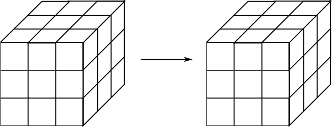
The MeldSpheres function computes the smallest sphere containing the initial two. If one is inside the other the result it the outer sphere. The resulting spheres could be larger than necessary to bound all contained objects. This overhead means that a search could test some spheres two much but statistically this will have no effect.
|
1 2 3 4 5 6 7 8 9 10 11 12 |
void MeldSpheres( Sphere& _S1, const Sphere& _S2 ) { Vec3 vC = _S2.vCenter - _S1.vCenter; float fDist = len( vC ); // The outer radius is the distance of the reference sphere center and the // new sphere edge which is on the opposide side of the seconds sphere's center. float fOuterRadius = max( _S1.fRadius, _S2.fRadius - fDist ); float fRadius = 0.5f * ( max( fDist + _S2.fRadius, _S1.fRadius ) + fOuterRadius ); // Move to new center _S1.vCenter = _S1.vCenter + vC * ((fRadius - fOuterRadius)/(fDist+0.000001f)); _S1.fRadius = fRadius; } |
Detection
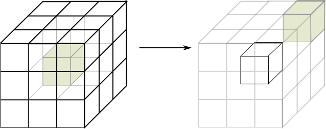
How to search for collisions in sphere tree? That is really easy! Take any geometry your basic collision test functions support and test recursively. If the current object collides with the sphere of the tree search in both children if possible. Otherwise we have a collision with a leaf i.e. with the bounding sphere of a certain object. Now the collision test between sphere and object must be performed e.g. on triangle level. Therefore the reference to the object is stored in the leaf node.
Now one last optimization should be mentioned. I have always spoken of objects, but what happens with large objects as terrains? They would always cause a triangle-level check if used as whole object. One option would be to split the terrain into more small parts. I used a much simpler version - an object in a tree leaf is either a sphere or a constant amount (2) of triangles. Once in a leaf the rest of the collision detection are two further primitive tests!
The switch from the brute force object-object test to the sphere tree saved ~2 milliseconds per frame (on my laptop with Core i5 3rd gen) while having one dynamic object.