Category Archives: Graphic

Description of rendering techniques

Volumetric Clouds and Offscreen Particles

At the end of 2012 and in January this year I played around with volumetric clouds. My first clouds I introduced in a rush where just big billboards with a value noise texture. I was relatively satisfied until a friend of mine came up with an improved billboard based approach in the game Skytides. He used Fourier Opacity Maps to compute volumetric shadowing. By the way this technique is very nice to get shadows for particles and other alpha blended objects. Now I was interested in real volumetric clouds in a real time context.

My first idea was to use ellipsoids and write a closed form ray casting which should be done in real time. Together with some noise they should form up single clouds. In the end the number of ellipsoids was limited and the quality bad.

So what comes next?

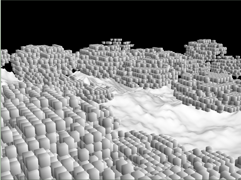
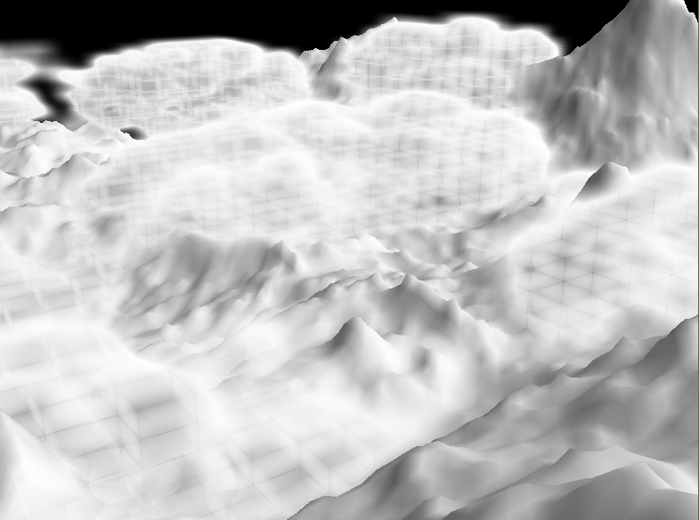
Ray tracing seemed to be the only promising step. I found some interesting stuff about cellular automatons for clouds by Dobashi. Nishita and co. So I tried to implement a ray marching on an integer texture where each bit is a voxel. In each voxel the boundary hit point to the next voxel can be computed in closed form too. This idea guaranteed an optimal step width but creates a very blocky look. I used dithering and interpolation which produced good quality results but was slow or too few detailed.

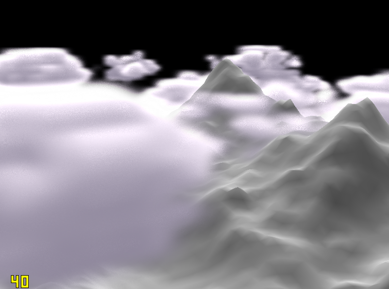
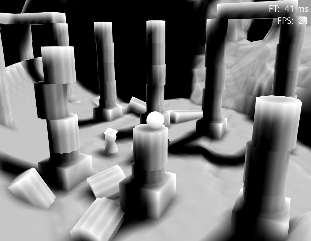
The last algorithm's results you see in the title bar of this page. It is so simple in its basics that you will hang me. The trick to get rid of block artefacts is to use fuzzy values and a linear sampler!

I use a standard ray marching (a for loop in the pixel shader) on a volume texture filled with a value noise. To animate the clouds I just move the texture around and sample twice at different locations.

To get clouds you need several rays: the fist ray accumulates the alpha values along the view direction. To get a volumetric lightning a ray into the lights direction is casted at each point which is not totally transparent. It took me some time to find a proper accumulation of alpha values. Assuming where 1 means an opaque value than must be computed per step on the ray. is the amount of background shining through the clouds. Finally the alpha value of a cloud is . There are different reasons to stop the ray casting:

The scene depth is reached (this makes things volumetric - of course the scene depth buffer is required)
The view distance is exceeded
is close to 0

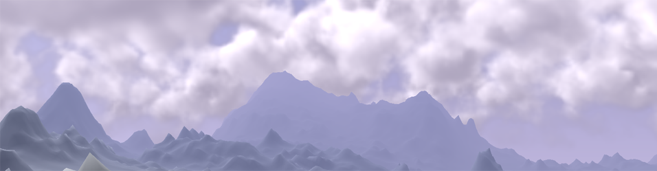
If you wanna have a good visual appearance this is enough! Stop reading her implement it and you will be done in a few hours.

Now comes the part of making things fast.

1. One ray into light direction per pixel on the primary ray - REALLY?
Yes! But no complete ray. I used a constant length ray of 6 steps. One might use the same alpha accumulation technique but just summing the density produces good results. The thing why this can work fast is to have relatively dense clouds. The primary ray is stifled after a few steps once it reaches a cloud. So there are not more light-castings than relevant.

2. What step size to choose?
The bigger the steps the fewer samples are necessary and everything gets faster and uglier. But in distance a small stepping ray is an overkill. I found a linear increasing step width ok.

3. Obviously clouds are smooth. They are so smooth you can put a 5x5 Gaussian filter onto it without seeing any difference. So why compute so many pixels with so expensive ray marching?
This part is the hardest and the reason for the "Offscreen Particles" in the title. All the nice things implemented so far could be computed on a 4 or 8 times smaller texture and than sampled up to screen size. I do not have screen shots of the upcoming problems when sampling alpha textures up but the GPU Gems 3 article has.
My solution works with only two passes the cloud pass and the upsampling. It is even not necessary to sample the z-buffer down.
The first pass renders the clouds to a small offscreen texture. It just fetches a single depth value at the current pixel position * 4 + 1.5. The 1.5 is more or less the centre of the represented area and must be changed if an other scaling factor than 4 is chosen. The output is: (Light intensity, Cloud Alpha, Sampled Z). The last component is the key. It remembers the actually used depth for later.
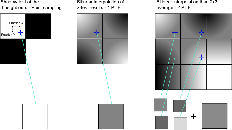
During the upsampling the linear interpolated texel from the cloud texture is taken. In case that (abs(Scene Z - Sampled Z) > threshold) the value taken from the clouds is not representative for the scenes pixel. This happens only at edges where we would get the artefacts. Now I take the 8 neighbourhood samples and search for the one with the smallest deviation from the scene depth. The so chosen representative is very likely a good approximation. There is no guarantee to find a better pixel but subjectively all artefacts are released. You might find some if directly searching for them. If someone has an idea how to do a more elegant search than you see in the shader below, please let me know.

In the following shader I used a doubled view distance and a distortion to get a better horizon. There also might be other not explained noise from other experiments.

#version 330

layout(std140) uniform Transformation {
    mat4 mView;
    mat4 mProjection;
    mat4 mViewProjection;
    mat4 mInverseViewProjection;
    vec3 vCameraPos;
    vec3 vCameraDir;
    float fNearClipPlane;
    vec3 vCameraUp;
    float fFarClipPlane;
};

layout(pixel_center_integer) in vec4 gl_FragCoord;
in vec3 vs_WorldPos;
uniform vec4 u_vParameter;		// (Voxel Density, Noise Threshold, 1-Noise Threshold, Scale)
uniform vec2 u_fPlanes;			// Lower and upper volume limit
uniform vec2 u_vHighToVolume;	// MAD transformation from World.y to [-1, 1] in the volume
uniform vec3 u_vColorBright;
uniform vec3 u_vColorDark;
uniform vec3 u_vWind1;
uniform vec3 u_vWind2;
uniform sampler3D u_Noise;
uniform sampler2D u_Depth;

const vec3 c_vLight = vec3( 0.707106, 0.707106, 0.0 );

out vec4 fs_Color;

// Density function.
float DensityFunction( vec3 _vPos )
{
    float fDensity = _vPos.y * u_vHighToVolume.x + u_vHighToVolume.y;
    fDensity = fDensity*fDensity;
    fDensity = - u_vParameter.y - fDensity*u_vParameter.z;
    float fAlpha = u_vParameter.x * max( 0, texture( u_Noise, _vPos * u_vParameter.w + u_vWind1 ).r + fDensity );
    fAlpha *= u_vParameter.x * max( 0, texture( u_Noise, _vPos.yxz * u_vParameter.w + u_vWind2 ).r + fDensity );
    return fAlpha;
}

// The ray marcher differs from the main one:
//	- stop after n steps, no depth test
//	- no alpha testing
//	- no call of lightocclusion
float lightocclusion( vec3 _vPos, vec3 _vDir )
{	
    float fDens = 1.0;

    for( int i=0; i<6; ++i)
    {
        // Next pos first - starting at the already sampled point.
        float fLen = 1.3;		// A little bit larger (light tends to produce less artefacts)
        _vPos += _vDir * fLen;

        fDens += DensityFunction( _vPos );
    }
    return fDens;
}

// Main ray marching function
// The step length is dynamic and depends linearly on depth.
vec3 density( vec3 _vPos, vec3 _vDir, vec3 _vLight, float _fZ )
{
    vec3 vRes = vec3( 1, 0, length( _vPos - vCameraPos ) );	// density, light and final depth

    float fRefY = _vDir.y;

    while( (_fZ > vRes.z) && ((_vPos.y-0.0001) < u_fPlanes.y) )
    {
        float fStepWidth = 0.6 + 0.006 * vRes.z;
        float fLen = min( _fZ-vRes.z, fStepWidth );

        float fAlpha = DensityFunction( _vPos ) * fLen;
        // Make clouds more transparent in the depth (instead of depth fog)
        fAlpha *= 1.0 - vRes.z / (2*fFarClipPlane);

        // Lightning
        if( fAlpha > 0.0001 )
        {
            vRes.y += fAlpha/lightocclusion( _vPos, _vLight ) * vRes.x;
            vRes.x *= 1 - fAlpha;

            // "Alphatesting"
            if( vRes.x < 0.004 ) return vec3( 0, vRes.y, vRes.z );
        }

        // 1 Use this line(s) to get a spherical effect at horizon
        _vDir.y = fRefY + 0.25 * max(0,vRes.z - fFarClipPlane) / fFarClipPlane;

        vRes.z += fLen;
        _vPos += _vDir * fLen;
    }

    return vRes;
}

void main(void)
{
    // Calculate the ray from camera through the cloud volume
    vec3 vDir = vs_WorldPos - vCameraPos;
    vDir = normalize( vDir );

    // The position is at least 4 times fNearClipPlane away from the camera (stability of plane transformation)
    // But ray should start at near plane.
    vec3 vStart = vs_WorldPos - 3.0f * fNearClipPlane * vDir;

    // Project into volume if outside y range
    float fMaxDist = fFarClipPlane-fNearClipPlane;
    float fProjDist = ( - max( vStart.y-u_fPlanes.y, 0 )) / vDir.y;
    if( u_fPlanes.x-vStart.y > 0 && vDir.y < -0.01 ) fProjDist = fMaxDist;
    vStart = vStart + fProjDist * vDir;

    // Where to end?
    ivec2 vTex = ivec2(gl_FragCoord.x*4+1.5, gl_FragCoord.y*4+1.5);
    float fZ = texelFetch( u_Depth, vTex, 0 ).r;
    // Compute linear depth from OpenGL projection
    float f_n = fFarClipPlane - fNearClipPlane;
    fZ = (- fFarClipPlane * fNearClipPlane / (fZ*f_n-fFarClipPlane));
    fZ = ( ( fZ >= fFarClipPlane ) ? (fFarClipPlane*2) : fZ );

    // If the ray hits the cloud volume
    vec3 vRes = density( vStart, vDir, c_vLight, fZ );

    fs_Color.r = vRes.y;
    fs_Color.g = (1-vRes.x);
    // The 0.5 is due to the fact that I compute clouds up to viewdistance*2
    fs_Color.z = 0.5 * fZ / fFarClipPlane;
}

100

101

102

103

104

105

106

107

108

109

110

111

112

113

114

115

116

117

118

119

120

121

122

123

124

125

126

127

128

129

#version 330

layout(std140) uniform Transformation {

mat4 mView;

mat4 mProjection;

mat4 mViewProjection;

mat4 mInverseViewProjection;

vec3 vCameraPos;

vec3 vCameraDir;

float fNearClipPlane;

vec3 vCameraUp;

float fFarClipPlane;

};

layout(pixel_center_integer) in vec4 gl_FragCoord;

in vec3 vs_WorldPos;

uniform vec4 u_vParameter; // (Voxel Density, Noise Threshold, 1-Noise Threshold, Scale)

uniform vec2 u_fPlanes; // Lower and upper volume limit

uniform vec2 u_vHighToVolume; // MAD transformation from World.y to [-1, 1] in the volume

uniform vec3 u_vColorBright;

uniform vec3 u_vColorDark;

uniform vec3 u_vWind1;

uniform vec3 u_vWind2;

uniform sampler3D u_Noise;

uniform sampler2D u_Depth;

const vec3 c_vLight = vec3( 0.707106, 0.707106, 0.0 );

out vec4 fs_Color;

// Density function.

float DensityFunction( vec3 _vPos )

{

float fDensity = _vPos.y * u_vHighToVolume.x + u_vHighToVolume.y;

fDensity = fDensity*fDensity;

fDensity = - u_vParameter.y - fDensity*u_vParameter.z;

float fAlpha = u_vParameter.x * max( 0, texture( u_Noise, _vPos * u_vParameter.w + u_vWind1 ).r + fDensity );

fAlpha *= u_vParameter.x * max( 0, texture( u_Noise, _vPos.yxz * u_vParameter.w + u_vWind2 ).r + fDensity );

return fAlpha;

}

// The ray marcher differs from the main one:

// - stop after n steps, no depth test

// - no alpha testing

// - no call of lightocclusion

float lightocclusion( vec3 _vPos, vec3 _vDir )

{

float fDens = 1.0;

for( int i=0; i<6; ++i)

{

// Next pos first - starting at the already sampled point.

float fLen = 1.3; // A little bit larger (light tends to produce less artefacts)

_vPos += _vDir * fLen;

fDens += DensityFunction( _vPos );

}

return fDens;

}

// Main ray marching function

// The step length is dynamic and depends linearly on depth.

vec3 density( vec3 _vPos, vec3 _vDir, vec3 _vLight, float _fZ )

{

vec3 vRes = vec3( 1, 0, length( _vPos - vCameraPos ) ); // density, light and final depth

float fRefY = _vDir.y;

while( (_fZ > vRes.z) && ((_vPos.y-0.0001) < u_fPlanes.y) )

{

float fStepWidth = 0.6 + 0.006 * vRes.z;

float fLen = min( _fZ-vRes.z, fStepWidth );

float fAlpha = DensityFunction( _vPos ) * fLen;

// Make clouds more transparent in the depth (instead of depth fog)

fAlpha *= 1.0 - vRes.z / (2*fFarClipPlane);

// Lightning

if( fAlpha > 0.0001 )

{

vRes.y += fAlpha/lightocclusion( _vPos, _vLight ) * vRes.x;

vRes.x *= 1 - fAlpha;

// "Alphatesting"

if( vRes.x < 0.004 ) return vec3( 0, vRes.y, vRes.z );

}

// 1 Use this line(s) to get a spherical effect at horizon

_vDir.y = fRefY + 0.25 * max(0,vRes.z - fFarClipPlane) / fFarClipPlane;

vRes.z += fLen;

_vPos += _vDir * fLen;

}

return vRes;

}

void main(void)

{

// Calculate the ray from camera through the cloud volume

vec3 vDir = vs_WorldPos - vCameraPos;

vDir = normalize( vDir );

// The position is at least 4 times fNearClipPlane away from the camera (stability of plane transformation)

// But ray should start at near plane.

vec3 vStart = vs_WorldPos - 3.0f * fNearClipPlane * vDir;

// Project into volume if outside y range

float fMaxDist = fFarClipPlane-fNearClipPlane;

float fProjDist = ( - max( vStart.y-u_fPlanes.y, 0 )) / vDir.y;

if( u_fPlanes.x-vStart.y > 0 && vDir.y < -0.01 ) fProjDist = fMaxDist;

vStart = vStart + fProjDist * vDir;

// Where to end?

ivec2 vTex = ivec2(gl_FragCoord.x*4+1.5, gl_FragCoord.y*4+1.5);

float fZ = texelFetch( u_Depth, vTex, 0 ).r;

// Compute linear depth from OpenGL projection

float f_n = fFarClipPlane - fNearClipPlane;

fZ = (- fFarClipPlane * fNearClipPlane / (fZ*f_n-fFarClipPlane));

fZ = ( ( fZ >= fFarClipPlane ) ? (fFarClipPlane*2) : fZ );

// If the ray hits the cloud volume

vec3 vRes = density( vStart, vDir, c_vLight, fZ );

fs_Color.r = vRes.y;

fs_Color.g = (1-vRes.x);

// The 0.5 is due to the fact that I compute clouds up to viewdistance*2

fs_Color.z = 0.5 * fZ / fFarClipPlane;

}

#version 330

layout(std140) uniform Transformation {
    mat4 mView;
    mat4 mProjection;
    mat4 mViewProjection;
    mat4 mInverseViewProjection;
    vec3 vCameraPos;
    vec3 vCameraDir;
    float fNearClipPlane;
    vec3 vCameraUp;
    float fFarClipPlane;
};

uniform vec2 u_vCloudRes;
uniform vec3 u_vColorCloudBright;
uniform vec3 u_vColorCloudDark;
uniform sampler2D u_Clouds;
uniform sampler2D u_Scene;
uniform sampler2D u_Depth;

in vec2 vs_TexCoord0;
in vec3 vs_WorldPos;
out vec4 fs_Color;

// ------------------------------------------------
// SKY
// ------------------------------------------------
const vec3 AdditonalSunColor = vec3(1.0, 0.98, 0.8)/2.5;
const vec3 LowerHorizonColour = vec3(0.815, 1.141, 1.54)/3;
const vec3 UpperHorizonColour = vec3(0.986, 1.689, 2.845)/3;
const vec3 UpperSkyColour = vec3(0.16, 0.27, 0.63);//*0.8;
const vec3 GroundColour = vec3(0.31, 0.41, 0.7)*0.8;
const vec3 LightDirection = vec3( 0.707106, 0.707106, 0.0 );
const float LowerHorizonHeight = -0.4;
const float UpperHorizonHeight = -0.1;
const float SunAttenuation = 2;
vec3 ComputeSkyColor( in vec3 ray )
{
    vec3 color;

    // background
    vec3 vExtraColor = u_vColorCloudDark * 1.3;
    float heightValue = ray.y;	// mirror..
    if(heightValue < LowerHorizonHeight)
    color = mix(GroundColour, LowerHorizonColour, (heightValue+1) / (LowerHorizonHeight+1));
	else if(heightValue < UpperHorizonHeight)
    color = mix(LowerHorizonColour, vExtraColor, (heightValue-LowerHorizonHeight) / (UpperHorizonHeight - LowerHorizonHeight));
	else
    color = mix(vExtraColor, UpperSkyColour, (heightValue-UpperHorizonHeight) / (1.0-UpperHorizonHeight));

    // Sun
    float angle = max(0, dot(ray, LightDirection));
    color += (pow(angle, SunAttenuation) + pow(angle, 10000)*10) * AdditonalSunColor;

    return color;//min(vec3(1,1,1), color);
}

void main()
{
    // Sample the cloud from low res picture (with 4 neighbourhood),
    // the scene and the depth
    vec3 vColorCloud0 = texture( u_Clouds, vs_TexCoord0 ).rgb;
    vec3 vColorScene = texture( u_Scene, vs_TexCoord0 ).rgb;
    float fZ = texture( u_Depth, vs_TexCoord0 ).r;

    // Transform Z and test again (this removes artefacts where clouds overlay
    // the scene).
    float f_n = fFarClipPlane - fNearClipPlane;
    fZ = 0.5 * (- fNearClipPlane / (fZ*f_n-fFarClipPlane));

    // Is it a background pixel?
    vec3 vRay = vs_WorldPos - vCameraPos;
    vec3 vBackColor = ComputeSkyColor( normalize( vRay ) );
    if( fZ >= 0.49999 )
    {
        vColorScene = vBackColor;
        fZ *= 2;
    } else
    {
        // depth fog
        vColorScene = mix( vColorScene, GroundColour, 2*fZ );
        vColorScene = mix( vColorScene, vBackColor, 4*fZ*fZ );
    }

    // Has current pixel totaly wrong depth?
    vec2 vLightDensity = vColorCloud0.rg;
    float fZError = abs(fZ - vColorCloud0.z);
    if( fZError > 0.01 )
    {
        // Choose the cloud sample, which has the best fitting depth.
        ivec2 vCloudTex = ivec2( u_vCloudRes * vs_TexCoord0 );
        vec3 vColorCloud1 = texelFetch( u_Clouds, vCloudTex+ivec2(-1, 0), 0 ).rgb;
        vec3 vColorCloud2 = texelFetch( u_Clouds, vCloudTex+ivec2( 1, 0), 0 ).rgb;
        vec3 vColorCloud3 = texelFetch( u_Clouds, vCloudTex+ivec2( 0,-1), 0 ).rgb;
        vec3 vColorCloud4 = texelFetch( u_Clouds, vCloudTex+ivec2( 0, 1), 0 ).rgb;
        vec3 vColorCloud5 = texelFetch( u_Clouds, vCloudTex+ivec2( 1, 1), 0 ).rgb;
        vec3 vColorCloud6 = texelFetch( u_Clouds, vCloudTex+ivec2( 1,-1), 0 ).rgb;
        vec3 vColorCloud7 = texelFetch( u_Clouds, vCloudTex+ivec2(-1, 1), 0 ).rgb;
        vec3 vColorCloud8 = texelFetch( u_Clouds, vCloudTex+ivec2(-1,-1), 0 ).rgb;

        vec4 vZEs = abs( vec4( fZ - vColorCloud1.z, fZ - vColorCloud2.z, fZ - vColorCloud3.z, fZ - vColorCloud4.z ) );
        vec4 vZEs2 = abs( vec4( fZ - vColorCloud5.z, fZ - vColorCloud6.z, fZ - vColorCloud7.z, fZ - vColorCloud8.z ) );
        vLightDensity = (vZEs.x < vZEs.y) ? vColorCloud1.rg : vColorCloud2.rg; fZError = min( vZEs.x, vZEs.y );
        vLightDensity = (vZEs.z < fZError) ? vColorCloud3.rg : vLightDensity; fZError = min( vZEs.z, fZError );
        vLightDensity = (vZEs.w < fZError) ? vColorCloud4.rg : vLightDensity; fZError = min( vZEs.w, fZError );
        vLightDensity = (vZEs2.x < fZError) ? vColorCloud5.rg : vLightDensity; fZError = min( vZEs2.x, fZError );
        vLightDensity = (vZEs2.y < fZError) ? vColorCloud6.rg : vLightDensity; fZError = min( vZEs2.y, fZError );
        vLightDensity = (vZEs2.z < fZError) ? vColorCloud7.rg : vLightDensity; fZError = min( vZEs2.z, fZError );
        vLightDensity = (vZEs2.w < fZError) ? vColorCloud8.rg : vLightDensity;
    }

    vec3 vFinalCloudColor = mix( u_vColorCloudDark, u_vColorCloudBright, vLightDensity.r );
    fs_Color.rgb = mix( vColorScene, vFinalCloudColor, vLightDensity.g );
    fs_Color.a = 1;
}

100

101

102

103

104

105

106

107

108

109

110

111

112

113

114

115

116

#version 330

layout(std140) uniform Transformation {

mat4 mView;

mat4 mProjection;

mat4 mViewProjection;

mat4 mInverseViewProjection;

vec3 vCameraPos;

vec3 vCameraDir;

float fNearClipPlane;

vec3 vCameraUp;

float fFarClipPlane;

};

uniform vec2 u_vCloudRes;

uniform vec3 u_vColorCloudBright;

uniform vec3 u_vColorCloudDark;

uniform sampler2D u_Clouds;

uniform sampler2D u_Scene;

uniform sampler2D u_Depth;

in vec2 vs_TexCoord0;

in vec3 vs_WorldPos;

out vec4 fs_Color;

// ------------------------------------------------

// SKY

// ------------------------------------------------

const vec3 AdditonalSunColor = vec3(1.0, 0.98, 0.8)/2.5;

const vec3 LowerHorizonColour = vec3(0.815, 1.141, 1.54)/3;

const vec3 UpperHorizonColour = vec3(0.986, 1.689, 2.845)/3;

const vec3 UpperSkyColour = vec3(0.16, 0.27, 0.63);//*0.8;

const vec3 GroundColour = vec3(0.31, 0.41, 0.7)*0.8;

const vec3 LightDirection = vec3( 0.707106, 0.707106, 0.0 );

const float LowerHorizonHeight = -0.4;

const float UpperHorizonHeight = -0.1;

const float SunAttenuation = 2;

vec3 ComputeSkyColor( in vec3 ray )

{

vec3 color;

// background

vec3 vExtraColor = u_vColorCloudDark * 1.3;

float heightValue = ray.y; // mirror..

if(heightValue < LowerHorizonHeight)

color = mix(GroundColour, LowerHorizonColour, (heightValue+1) / (LowerHorizonHeight+1));

else if(heightValue < UpperHorizonHeight)

color = mix(LowerHorizonColour, vExtraColor, (heightValue-LowerHorizonHeight) / (UpperHorizonHeight - LowerHorizonHeight));

else

color = mix(vExtraColor, UpperSkyColour, (heightValue-UpperHorizonHeight) / (1.0-UpperHorizonHeight));

// Sun

float angle = max(0, dot(ray, LightDirection));

color += (pow(angle, SunAttenuation) + pow(angle, 10000)*10) * AdditonalSunColor;

return color;//min(vec3(1,1,1), color);

}

void main()

{

// Sample the cloud from low res picture (with 4 neighbourhood),

// the scene and the depth

vec3 vColorCloud0 = texture( u_Clouds, vs_TexCoord0 ).rgb;

vec3 vColorScene = texture( u_Scene, vs_TexCoord0 ).rgb;

float fZ = texture( u_Depth, vs_TexCoord0 ).r;

// Transform Z and test again (this removes artefacts where clouds overlay

// the scene).

float f_n = fFarClipPlane - fNearClipPlane;

fZ = 0.5 * (- fNearClipPlane / (fZ*f_n-fFarClipPlane));

// Is it a background pixel?

vec3 vRay = vs_WorldPos - vCameraPos;

vec3 vBackColor = ComputeSkyColor( normalize( vRay ) );

if( fZ >= 0.49999 )

{

vColorScene = vBackColor;

fZ *= 2;

} else

{

// depth fog

vColorScene = mix( vColorScene, GroundColour, 2*fZ );

vColorScene = mix( vColorScene, vBackColor, 4*fZ*fZ );

}

// Has current pixel totaly wrong depth?

vec2 vLightDensity = vColorCloud0.rg;

float fZError = abs(fZ - vColorCloud0.z);

if( fZError > 0.01 )

{

// Choose the cloud sample, which has the best fitting depth.

ivec2 vCloudTex = ivec2( u_vCloudRes * vs_TexCoord0 );

vec3 vColorCloud1 = texelFetch( u_Clouds, vCloudTex+ivec2(-1, 0), 0 ).rgb;

vec3 vColorCloud2 = texelFetch( u_Clouds, vCloudTex+ivec2( 1, 0), 0 ).rgb;

vec3 vColorCloud3 = texelFetch( u_Clouds, vCloudTex+ivec2( 0,-1), 0 ).rgb;

vec3 vColorCloud4 = texelFetch( u_Clouds, vCloudTex+ivec2( 0, 1), 0 ).rgb;

vec3 vColorCloud5 = texelFetch( u_Clouds, vCloudTex+ivec2( 1, 1), 0 ).rgb;

vec3 vColorCloud6 = texelFetch( u_Clouds, vCloudTex+ivec2( 1,-1), 0 ).rgb;

vec3 vColorCloud7 = texelFetch( u_Clouds, vCloudTex+ivec2(-1, 1), 0 ).rgb;

vec3 vColorCloud8 = texelFetch( u_Clouds, vCloudTex+ivec2(-1,-1), 0 ).rgb;

vec4 vZEs = abs( vec4( fZ - vColorCloud1.z, fZ - vColorCloud2.z, fZ - vColorCloud3.z, fZ - vColorCloud4.z ) );

vec4 vZEs2 = abs( vec4( fZ - vColorCloud5.z, fZ - vColorCloud6.z, fZ - vColorCloud7.z, fZ - vColorCloud8.z ) );

vLightDensity = (vZEs.x < vZEs.y) ? vColorCloud1.rg : vColorCloud2.rg; fZError = min( vZEs.x, vZEs.y );

vLightDensity = (vZEs.z < fZError) ? vColorCloud3.rg : vLightDensity; fZError = min( vZEs.z, fZError );

vLightDensity = (vZEs.w < fZError) ? vColorCloud4.rg : vLightDensity; fZError = min( vZEs.w, fZError );

vLightDensity = (vZEs2.x < fZError) ? vColorCloud5.rg : vLightDensity; fZError = min( vZEs2.x, fZError );

vLightDensity = (vZEs2.y < fZError) ? vColorCloud6.rg : vLightDensity; fZError = min( vZEs2.y, fZError );

vLightDensity = (vZEs2.z < fZError) ? vColorCloud7.rg : vLightDensity; fZError = min( vZEs2.z, fZError );

vLightDensity = (vZEs2.w < fZError) ? vColorCloud8.rg : vLightDensity;

}

vec3 vFinalCloudColor = mix( u_vColorCloudDark, u_vColorCloudBright, vLightDensity.r );

fs_Color.rgb = mix( vColorScene, vFinalCloudColor, vLightDensity.g );

fs_Color.a = 1;

}

All together this runs with >50 fps on my laptop's Intel chip - in full HD:

Faster PCF

PCF Shadow Acne

Solution Attemps (working for other sampling techniques)

Shadow acne is a common artifact in shadow map techniques. Similar to z-fighting artifacts some sharp-edged shadow appear on surfaces which should not be shadowed at all. This effect emerge if the surface tangential plain and the light direction are nearly parallel.

Shadows only - Artifacts at surfaces and behind the "player" (middle)

The image shows the shadows of a 4x4 PCF sampled shadow map. For the demonstration a coarse resolution of 1024x1024 was used for the whole scene and objects's front sides were drawn into it. The sphere in the middle only occupies 4 texels in the shadow map.

z-fighting: Even without PCF you can observe such streak patterns. This happens if the z values are very similar and the test fails due to precision errors or because the z buffer represents the value of a wrong pixel (e.g. some neighbour). A continuous map would solve this problem...

Solution 1: Offsetting
Often one subtract a constant value from the shadow map before comparing it to the current z value. This succeeds if the light is perpendicular to the surface. If they are not we get a new problem. Since point sampling chooses one or the other sample a pixel, a pixel in between is not represented properly. The smaller the angle between light and tangential plain the larger the difference of neighboured pixels in the shadow map. The consequence is that the offset needs to be much larger to avoid a wrong in-shadow-classification for the non represented points. Moreover the offset depends on the normal. One drawback of a larger offset is a new artifact called peter panning which is a gab between an object an its shadow.
→ Can be helpful if the offset is chosen depending on the normal, otherwise this is crap.

PCF on an interpolated Z-buffer.

Solution 2: Interpolating the Shadow Map

Yes, we can sample the shadow map with the standard linear sampler. This is correct if the surface between the two points in the shadow map is plain which it is most times. The gain of this is great and all artifacts are removed - for small samplers. Unfortunately this cannot be applied to PCF, because there we need the fraction of the pixel position for smoothing the shadow.
→ Solution for hard edged shadow sampling. Cannot be applied to PCF

Solution 3: Back faces and Offset-Meshes
Until now I have drawn front faces during the shadow map creation pass. Using back faces helps against z-fighting because the front faces always have a large offset to the back of the same model. Similar the mesh could be pumped along the normals to create a surface considering offset. This technique succeeds if the back faces are recognized as always in shadow. I would like to apply lighting to back faces too, so this would only move artifacts to the back side and causes further problems with self shadowing.
I did not tested Offset-Meshes which could be a good solution even for my scenario.

Comparision of and *0.5+0.5 (No ambient and other lighting) - Back faces on the left are "flat"

Comparison of <N,L> and <N,L>*0.5+0.5 (No ambient and other lighting) - Back faces on the left are "flat"

Now the PCF Sampling technique introduces an additional problem with the z-values. That we use the same interpolation factors is ok, but that we use the same z-value for the lookup of neighbours creates a lot of shadow acne. Moreover the direction in which we look on our neighbours is in light space! it would be better to go steps in the object space and transform that positions to light space. However this is the reason for an increase of artifacts.

The overall quality of PCF is good and supported by modern hardware. HLSL offers an intrinsic to do the lookup and the interpolation, or to fetch 4 pixel with the Gather command which I used in the code below.
Unfortunately none of the mentioned solutions 1-3 work for that kind of sampling (see pictures).

Solution (4) applied in Pathfinder

One mad+mul later

In graphics everything is a trick. Why bother with a correct algorithm if we can retouch the artifacts.
Observation: Obviously there is a boundary between some pixels where the z-lookup on the one side is very different from the one on the other side (→ streaks/banding). Close to this boundary the z-values must be very similar. I liked to smooth this boundary. My idea is to use the distance from the current z-value to the shadow map to find those edges. The distance must be small, because the values are very similar in the problem regions and lie on both sides of the shadow map value. So I multiply the shadow value with a clamped distance to get a linear decrease of light close to the boundary (see highlighted code).

PCF 3x3 (No other lighting!), coarse map resolution (remember the sphere in the middle gets only 4 texels in the shadow map)

In consequence everything gets darker. For each point visible from the light the distance to the shadow map value is more or less 0. The whole scene would get black without the offset in line 33. This whole trick only requires two instructions for each lookup (mad_sat and mul). I replaced the streak artifacts by a new underexposure artifact. Well done! If you look on the results you will be satisfied. The new artifacts behaves a little bit like ambient occlusion. Yes, I got a very cheap ambient occlusion where other people use complex algorithms for ;-). But the higher the shadow map resolution the less this artifact appears. So I lost this nice side effect as I switched to cascaded shadow maps and increased the resolution.

// Compute the fraction of the coordinate and 1-x_frac, ...
// With these factors a bilinear interpolation can be done with one
// dp4 (dot product).
// The order of the returned factors matches the pixel order of the
// Gather command: (1-x)*(1-y), x*(1-y), (1-x)*y, x*y
float4 bilinearFactors( float2 _vCoord )
{
    float4 vFrac;
    vFrac.xy = frac(_vCoord);
    vFrac.zw = 1-vFrac.xy;
    return vFrac.zxzx*vFrac.wwyy;
}

// Perform a parallel lookup of 4 shadow values and do a "corrected"
// interpolation in between.
float shadowLookup( Texture2D _ShadowMap, float2 _vCoord, float _fZ, float _fZScaled, float4 _vFrac, int2 _vOffset )
{
    // Sample and compare
    float4 vDepthSamples = _ShadowMap.Gather( g_PointSampler, _vCoord, _vOffset );
    float4 vShadows = vDepthSamples > _fZ;
    // "Correction" of hard z-test edges.
    vShadows *= saturate(vDepthSamples*2048.0 - _fZScaled);
    // Interpolation
    return dot( vShadows.wzxy, _vFrac );
}

// Compute the shadow value in [0,1] for the given postion
float computePCFShadow3( Texture2D _ShadowMap, float3 _vWorldPos )
{
    float3 vLightSpaceCoord = mul(float4(_vWorldPos, 1), c_mLightViewProjection).xyz;
    // Is the current sample in the shadowmap or outside the volume?
    // Blend decreases the shadow intensity to the edges of the shadowmap.	
    vLightSpaceCoord = vLightSpaceCoord*float3(0.5,-0.5, 1.0)+float3(0.5, 0.5, -0.0005);

    // perform PCF filtering on a 3 x 3 texel neighborhood
    float fSum = 0.0f;
    float4 vInterpolationFactors = bilinearFactors( vLightSpaceCoord.xy*c_fShadowMapResolution-0.5 );
    float fZScaled = vLightSpaceCoord.z * 2048.0;
    for( int y = -1; y <= 1; y++ )
        for( int x = -1; x <= 1; x++ )
            fSum += shadowLookup(_ShadowMap, vLightSpaceCoord.xy, vLightSpaceCoord.z, fZScaled, vInterpolationFactors, int2(x,y));
    return lerp( fSum/9.0, 1, fBlend);
}

// Compute the fraction of the coordinate and 1-x_frac, ...

// With these factors a bilinear interpolation can be done with one

// dp4 (dot product).

// The order of the returned factors matches the pixel order of the

// Gather command: (1-x)*(1-y), x*(1-y), (1-x)*y, x*y

float4 bilinearFactors( float2 _vCoord )

{

float4 vFrac;

vFrac.xy = frac(_vCoord);

vFrac.zw = 1-vFrac.xy;

return vFrac.zxzx*vFrac.wwyy;

}

// Perform a parallel lookup of 4 shadow values and do a "corrected"

// interpolation in between.

float shadowLookup( Texture2D _ShadowMap, float2 _vCoord, float _fZ, float _fZScaled, float4 _vFrac, int2 _vOffset )

{

// Sample and compare

float4 vDepthSamples = _ShadowMap.Gather( g_PointSampler, _vCoord, _vOffset );

float4 vShadows = vDepthSamples > _fZ;

// "Correction" of hard z-test edges.

vShadows *= saturate(vDepthSamples*2048.0 - _fZScaled);

// Interpolation

return dot( vShadows.wzxy, _vFrac );

}

// Compute the shadow value in [0,1] for the given postion

float computePCFShadow3( Texture2D _ShadowMap, float3 _vWorldPos )

{

float3 vLightSpaceCoord = mul(float4(_vWorldPos, 1), c_mLightViewProjection).xyz;

// Is the current sample in the shadowmap or outside the volume?

// Blend decreases the shadow intensity to the edges of the shadowmap.

vLightSpaceCoord = vLightSpaceCoord*float3(0.5,-0.5, 1.0)+float3(0.5, 0.5, -0.0005);

// perform PCF filtering on a 3 x 3 texel neighborhood

float fSum = 0.0f;

float4 vInterpolationFactors = bilinearFactors( vLightSpaceCoord.xy*c_fShadowMapResolution-0.5 );

float fZScaled = vLightSpaceCoord.z * 2048.0;

for( int y = -1; y <= 1; y++ )

for( int x = -1; x <= 1; x++ )

fSum += shadowLookup(_ShadowMap, vLightSpaceCoord.xy, vLightSpaceCoord.z, fZScaled, vInterpolationFactors, int2(x,y));

return lerp( fSum/9.0, 1, fBlend);

}

Developerblog – Johannes Jendersie

Content Generators & Demos