Category Archives: Generators

Creation of models and textures through pure code

Labyrinth Generation

This weekend I wrote a simply labyrinth generator for Pathfinder. It is surprisingly easy to get interesting systems. Much easier than trees!

labyrinth

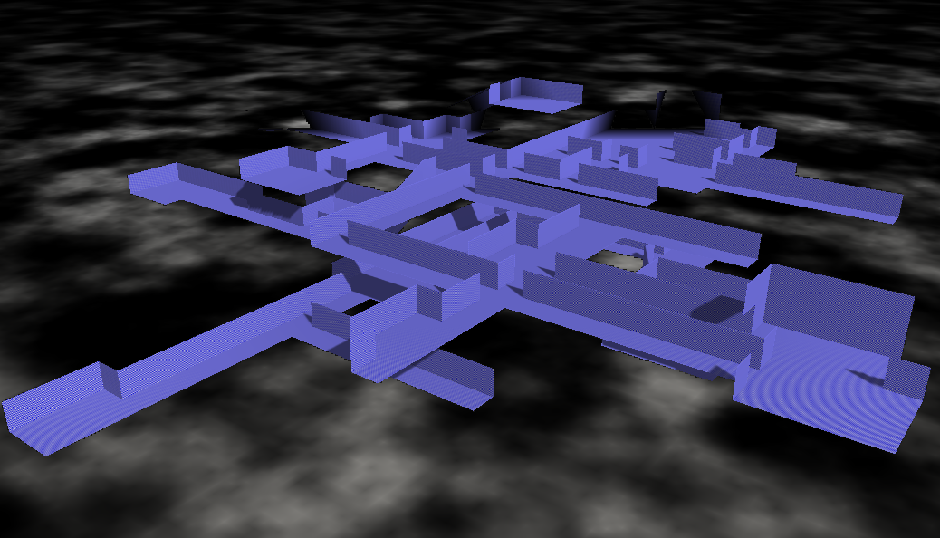
The first and most important decision I made was to use a voxel grid. To create a mesh immediately would cause problems with self intersections. So my idea was to create a volume texture and just set voxels to solid, corridor, stairs, ... After that one could use a standard extraction of implicit surfaces (Marching Cubes or Dual Contouring). I decided to use a specialised generator to hold the amount of triangles low.

Without the special case of stairs the idea is very simple: For each non-solid voxel sample its 6 neighbours. If there is a solid voxel there must be a wall on that side - create a quad.

Component Generator

The generator must fill the voxel grid with meaningful values now. Since I would like to have corridors and rooms and no natural shapes it is sufficient to use very large voxels where one single voxels is already a corridor/room.

I divided the generator itself into two parts: The single components to describe a certain structure and a recursive method to create the full labyrinth. Each of the component generators return a position where further creations could be attached. My generator uses 3 basic elements:

  • Corridors: Just set a line of voxels to "Corridor". A corridor has a random length in [2,10].
  • Chambers: Create a larger empty volume centered at the entrance.
  • Stairs: Create two diagonal voxels of type stair. The problem here is the triangulation.Laby_Stairs There should be a slope between two floors but so far only axis aligned triangles are generated. I introduced a shearing for the stair voxels. So far so good but the resulting corridor will cross solid voxels (see image). That itself is no problem, but if an other structure intersects there this will cause an ugly triangle inside the room. To overcome this a stair structure locks its surrounding as solid.
    An much easier approach would be to create vertical corridors and insert stairs as extra objects. It is a design decision that I would like to have these slopes.

The recursive part is doing the following thing: Chose one of the structures probabilistically. If it is "corridors" create 1-3 corridors, otherwise create exactly one of the chosen structure. Continue recursion at each returned attachment point. To stop the recursion a counter is decreased in each step. It does not directly count the recursion depth. Instead it is decreased by the number of created sub-structures. So if there are 3 corridors the counter is decreased faster to stop the recursion earlier. This should stabilize the "size" of the result. For a really stable size-controll-factor it would be necessary to divide the remaining number through the number of sub calls. On that way one could exactly create n structures where n is given in advance.

It should be said that the generator can create labyrinths of where different complexity. In the described approach floors are generated in each voxel grid level. There are many points where the structures intersect vertically. It is possible to jump down into the floor below and there are even circles in 3D where the common rule "always touch the wall with the same hand" does not succeed to leave the labyrinth. To make things easier I create stairs of length two so one voxel level is always skipped. Due to chambers it is still possible that there are vertical intersections but they are rare.

In conclusion it was a very good idea to use voxels in the first place. In feature I might use the component based generator approach for other things. One could even think of something hierarchically. For each substructure one can just ignore everything else and concentrate on a meaningful result.

Example Rule: The Redwood Tree

In order to make the core of Voxel Seeds more understandable I would like to explain two generic rules which together create the oak tree.

Each tree is build upon two rules - one for the wood and one for the leaves/needles. Thinking of a real automaton there are much more rules, but considering the form explained in About the automaton behind Voxel Seeds allows branching inside a rule. This is why I refer to generic rules.

As mentioned in the last post about the automaton we added a small memory to each living voxel. The first one was a "Tick" counter. This is some stopwatch when to apply the rule next. Each species has its own intervall length determining the growth speed. Further this counter can be manipulated randomly to break the synchronous growth.

The redwood has the mightiest rule allowing a procedural fractal tree. Lets start with the needles first. The rule is called SphericalLeafRule and is used for oak trees and redwoods. The idea is to seed a center voxel of the needle/leaf type and do a flood-fill of a spherical region. How can the euclidean distance to the center be estimated? This question is answered later for the redwood itself. For needles it is sufficient to use some random manhatten like distance. Therefore the "Generation" memory is used. This is monotonously increasing and the growth stops if the number gets too large. Here is some pseudo code of the rule:

To compute the euclidean distance to some center voxel a little bit more work has to be done. It is possible to store a relative position into a single 32 bit integer value. So one of the two memories could be used to store the center's position relative to the current voxel. If a new voxel is created in the neighbourhood it is easy to add or subtract one from the position to compute the new relative position. With this information each voxel can compute its euclidean distance to some source or destination point.

Now we have the ingredents for a  RedWoodRule . First of all the "Generation" can be used to distinguish voxels of the same type but with a different growth behavior. The first important type is the kernel voxel c. The trunk and each branch consists of one line of these. When spawning a new kernel voxel it gets an encoded target in the "Resource" memory. Afterward these voxels try to reproduce into target direction. This is done randomly where the most probable chosen direction is that where the difference to the target is largest. During that growth new kernel voxels are created tangential to the chosen direction to build branches. If the growth reaches the target it creates a center voxel for the needles.
The second type is the raw wood r. These have a "Generation" counter larger than 1000 where the difference to 1000 describes the target width of the trunk/branch. For each kernel voxel the width is determined by the distance to its target. If this width is at least one r voxels are spawned in the neighbourhood. These remember there spawner position in the "Resource" field and growth further if they are not too far away. I.e. if the stored width from the "Generation" counter is larger than there actual euclidean distance. In general this creates a sphere for a single kernel voxel filled with wood. The sum of many such neighboured spheres creates a cylinder. The advantage in contrast to a real cylinder is that twists in the kernel line do not cause holes in the surrounding.

The MST Distance Field

Distance field of a convex polygon

Distance field of a convex polygon

First of all: what is the gain of using distance fields for terrain generation? A distance field is the image of a distance function where black is very close to some object and white is far away. The results differ for different shaped objects as points or lines.
Well, using a 2D distance field as a 2D height map will create mountains or bubbles or cells depending on the objects' shape and the distance function to the objects. Everything in this post is using the euclidean distance .
As I had seen a picture like the one on the right side first I had thought "It looks like a mountain".

The second thing I observed was that minimal spanning trees (MST) of point sets where all points are connected to each other looks very much like a maintain ridge chain.

Alps height map (reality)

Alps height map (reality)

Distance to MST of 100 uniform distributed points

Distance to MST of 100 uniform distributed points

The nice thing you can see on the right picture is that the distance field is "height" where much space is available. So there are height and small mountains mixed and the result is a nice base shape for a terrain.

One problem of using a distance function is that outside (not on the image) the distance will increase further and further. So the mountains do end in a plane but in a limited high plateau around the MST region. This leads to the idea of using the inverse: .

Inverse distance of the same MST as in the previous picture

Inverse distance of the same MST as in the previous picture

An advantage of the inverse function is that our initial points are now the highest points = summits. On the other hand the whole MST has the same height! All ridges and summits are on the same level now. Before all valleys had a height of 0 which was less visible.

Consider the nice property that the points are the summits. It is now very intuitive to give each point an individual height and somehow change the distance function.

All test to change the distance function itself produced artifacts. It will always make problems because the result is a global property which may depend on all vertices and edges of the MST graph.

To solve that issue I took a global interpolation scheme to compute the local height and multiplied the results with the pure distance field which works great!

Computation of the distance field

There are lots of papers related to this issue. Assuming point objects everywere and make a straight forward convolution of a map would take time. There are better ways to do that with a point map, but I thought about using the graph itself. Then the computation takes where is the number of edges in the MST which I assumed to be relatively small. It is not possible to go beyond because we have to write each pixel at least once. For an implementation example of a point-line distance function see my collection of functions (TODO).

To compute the parametrised height I used a weighted mean:


where is a radial basis function. The farther the point is away the less it contributes to the current height. I found the Gaussian RBF and the Inverse Quadric RBF to be useful.